Temperature Control 1: Simple Control Theory

Posted : 2 weeks, 6 days ago

Temperature Control

The need to control temperature is everywhere, but getting it right is more difficult than one might expect. A domestic furnace controlled by a simple thermostat keeps a house comfortable in winter, but the inside air temperature swings irregularly over a range of a few degrees. That's fine for a house---you can have a New Year's party, with a bunch of people dissipating a hundred watts each, doors to hot ovens and the cold outside opening and closing, no worries whatsoever.  The heating system keeps it comfortable.

Such sloppy control doesn't work everywhere.  In applications such as scientific instruments, industrial process control, tunable diode lasers, bioreactors, and high precision mechanisms, we often need much better. It's far from rare for them to need temperature control down to the millikelvin or even microkelvin range. For that, we need a better control system: tighter error limits, higher speed, and higher precision.  (And usually higher accuracy, but that's a point we'll leave for later.)

Temperature control is a complicated multidimensional problem, because we usually want to minimize temperature transients and gradients in some object, as well as keeping its average temperature constant.  In this installment, we'll develop a few control system ideas on a simpler system: a linear voltage regulator such as the familiar LM317, which has one input and one output.

Control System Example: A Linear Voltage Regulator

Probably the most popular adjustable voltage regulator of all time is the three-terminal LM317, which illustrates all the basic aspects of a control system.;

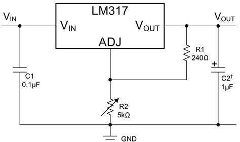
Figure 1: The Texas Instruments LM317 adjustable regulator (from the datasheet with a few annotations): a functional block diagram, followed by a simple application circuit.

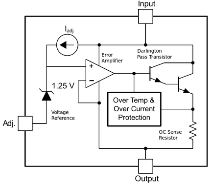
The job of the control loop is to make the output voltage follow the setpoint and resist external forcing from changes in supply voltage and load current.  The designer's job is to see that it does it well.  

A key concept in control systems is the plant, which is the thing the control loop controls, and consists of the process and the actuator. In the voltage regulator example, the plant is the combination of the power source and pass transistor (the actuator) with the output reservoir capacitor C2 and whatever load is attached (the process).  The controller  is what does the actual controlling, as one might expect.  

In this case it's the voltage reference, the  error amplifier, and the feedback divider R1/R2.  The feedback network forms

V_ADJ = V_OUT · R2 / (R1 + R2).                                                      (1)

The error amplifier takes the difference between V_ADJ and  V_OUT -1.25 V and  applies an amplified version to the base of the Darlington pass transistor, forming an overall feedback loop.  If the loop is stable, the error amplifier's gain is sufficiently high, and the resistors are small enough that we can ignore I_adj (~50 μA), the output will be very close to the setpoint defined by the reference and feedback network, 

V_nom =  V_ref · (R1 + R2) / R1 .                                                       (2)

The way this actually works is that the error amplifier multiplies the voltage difference V_err between the inputs by its gain AV_amp:

V_amp = AV_amp (V₊ – V_– ) = AV_amp V_err.                                         (3)

Thus it never quite gets to V_nom–there's always a bit of gain error, of order R2 /(AV_amp R1), which is generally less than the tolerance of the reference voltage (±4% for the LM317).

Open-Loop Behavior

We can investigate the control loop's operation by cutting it open, at least in thought.  This might seem like a weird thing to do, but it turns out to be the key move in understanding how the loop works.  Say we have an ideal version of the 317, where the Darlington has zero offset between base and emitter, rather than 2V_BE ~1.4V, so that the nominal amplifier output V_amp equals the unloaded V_out.  It'll simplify our discussion if we notionally attribute Zout to the final stage of the amplifier, and take the cut point to be right before that.  (Even a Darlington can load down one of those tiny on-chip amplifiers, and it's convenient to lump all the loading effects together.)  

We freeze the input to the final.  Its output will continue normally, except that there will be no feedback action to reduce the output impedance Z_out.  When a small increase in load current ΔI_load comes along, the output will sag a bit,

Vout = V_amp + V_sag, where V_sag = –Z_out ΔI_load.                            (4). 

This will change the voltage at the adjust pin by

ΔV_adj = V_sag  ·  R1/(R1 + R2),                                                       (5)

and the amplifier multiplies this by its inverting gain –A_Vamp,

ΔV_amp = – ΔV_adj ·  A_Vamp,                                                             (6)

so 

Once the feedback loop is closed again, the error amplifier is free to work, so it fights the voltage sag.   We can combine these to get an implicit expression for V_out,

V_out = A_Vamp·  (Vref  – V_out· (R1+R2)/R1) +V_sag,                          (7)

so

V_out = (A_Vamp· Vref +V_sag) /  ( 1 + A_Vamp · R1/ (R1 + R2) ) .         (8)

The second term in the denominator of  is the loop gain, which in open-loop terms is the gain from the final stage's input back to the output of its driver.

A_VL = A_Vamp· R1/(R1+R2)                                                             (9)

Since A_Vamp is complex-valued in the frequency domain, we see that depending on the phase, the denominator can vanish where |A_VL| = 1.  This turns out to dominate the behavior of the feedback system near equilibrium.  (Huge transients such as turn-on can cause nonlinear problems such as windup, which we'll get to in a later installment.)

Dividing top and bottom by A_Vamp, we get the more usual form of (8), 

V_out = (Vref +V_sag / A_Vamp) /  ( 1/ A_Vamp + R1/ (R1 + R2) ) ,         (10)

where we see that V_sag is suppressed by the amplifier gain.  If we assume A_Vamp  is very large, we recover the expression (2) for the nominal output voltage.

If the loop gain is 10, feedback will reduce the effect of load forcing by about 11 times compared with the open-loop value; if it is 1000, by 1001 times. (A_Vamp has some nonzero phase angle except at DC, so the factor probably isn't exactly 1/11 or 1/1001.)  So in general, having more loop gain is better.

How much we can actually use depends on the bandwidth of the error amplifier and on how fast the pass transistor can charge up the output reservoir capacitor.  

Due to the limitations of available components, the bandwidth of the feedback loop is finite, and different parts of it have different speed limitations; for instance, it is easier to make a fast amplifier than a fast, high-current pass transistor with low voltage drop.

In the next installment, we'll talk about frequency compensation, the gentle art of trading off speed, gain, and stability to get the best performance available.

• ← A High-Performance Time Domain Reflectometer
• "Super-Regenerative Receivers" by J. R. Whitehead →